
How to Treat Bitcoin ETF Inflows as a Testable Trading Signal (with a Trade Strategy template)
Turn Bitcoin ETF inflows into a repeatable experiment: source flows, design falsifiable hypotheses, backtest with realistic costs, and use Trade Strategy to document and compare results. Includes a downloadable experiment template.

# How to Treat Bitcoin ETF Inflows as a Testable Trading Signal (with a Trade Strategy template)
A sustained $1B+ seven-session inflow streak into Bitcoin ETFs is more than a headline — it can mark a temporary shift in momentum, liquidity and execution risk. For traders and quants, the productive response is not to assume a fixed edge but to turn the observation into a repeatable experiment.
This walkthrough presents a practical four-step process you can use to treat Bitcoin ETF inflows as a testable signal: (1) sourcing flow time series, (2) designing falsifiable hypotheses, (3) running external analyses and backtests, and (4) documenting outcomes using Trade Strategy’s released features (strategy management, historical results journal, strategy comparison). A downloadable experiment template is available on our blog.
## 1) Source a clean ETF flow time series
What you need
- Time series with a consistent timestamp (daily is common for ETF flows).
- Fields: date, net flow (USD), cumulative AUM, share changes where available.
- Synchronized BTC price series (same timezone and close times).
Practical sources and checks
- ETF issuers and regulatory filings often publish daily flows or AUM snapshots.
- Market-data vendors and research sites aggregate fund flows; use them where licensing permits.
Data hygiene checklist
- Align timestamps (e.g., ETF flows reported as "end-of-day" vs. BTC price close).
- Fill missing dates explicitly (mark as 0 flow or NaN depending on source semantics).
- Convert flows to consistent units (USD or BTC-equivalent) if you plan cross-asset comparisons.
Example: ingest and align (conceptual)
- Load ETF CSV: date, net_flow_usd, aum_usd
- Load BTC OHLC daily series
- Merge on date, forward-fill AUM if appropriate
Pseudocode (pandas-style):
```python
etf = pd.read_csv('etf_flows.csv', parse_dates=['date'])
btc = pd.read_csv('btc_daily.csv', parse_dates=['date'])
series = etf.merge(btc, on='date', how='inner')
series['flow_pct_of_aum'] = series['net_flow_usd'] / series['aum_usd']
```
Avoid making the flow series a black box — record the original provider and any cleaning steps you apply.
## 2) Design falsifiable hypotheses and trading rules
Think in terms of crisp, testable statements. Examples:
- H1 (momentum): "After a 3+ session streak of net inflows > $500M total, BTC exhibits positive average returns over the next 1–3 trading days."
- H2 (volatility): "Sustained inflow streaks compress realized intraday volatility over the following week due to incremental liquidity."
- H3 (execution risk): "Large inflow streaks widen bid-ask spreads on execution venues during the streak, increasing slippage for market orders."
Convert each hypothesis into a rule for backtesting
- Define a streak: minimum consecutive sessions and minimum cumulative flow.
- Define signal timing: enter at next-day open, or at close-of-day after the qualifying session.
- Define sizing and risk filters: position sizing, stop-loss, max daily notional.
- Define control groups: randomized entry dates or matched days without inflow streaks.
Parameterize for exploration (examples)
- Streak length: 2, 3, 5 days
- Flow threshold: $100M, $500M, $1B cumulative
- Lookahead: 1-day return, 3-day return, 7-day volatility
Keep hypotheses narrow so they’re easy to falsify and iterate.
## 3) Run external analysis and backtests (what to measure)
Recommended analyses
- Event study: compute average returns and confidence intervals for windows around qualifying streaks.
- Regression: include ETF flow magnitude and controls (BTC trend, realized vol) to check incremental explanatory power.
- Backtest: implement the trading rule and measure returns, risk-adjusted metrics, drawdowns and turnover.
Practical backtest considerations
- Slippage and market impact: use conservative assumptions for fills during high-flow periods.
- Transaction costs: include realistic fees and spread assumptions.
- Out-of-sample testing: reserve a recent period for validation.
Metrics to report
- Cumulative return and annualized return
- Sharpe or similar risk-adjusted metric
- Max drawdown and drawdown duration
- Number of signals and average trade duration
- Sensitivity to parameter choices
A quick event-study example (conceptual)
- For each streak date, compute BTC returns from T+1 to T+3.
- Aggregate across events and compare to bootstrapped control samples.
Note: do not rely on a single metric. If the signal performs only in-sample or is highly sensitive to thresholds, treat it cautiously.
## 4) Use Trade Strategy to document, monitor and compare experiments
Trade Strategy includes released features that help you turn analysis into a repeatable experiment. In particular, users can create and organize trading strategies, record and monitor historical strategy results, and compare strategies using saved information and historical results.
How to map the experiment to the platform
- Strategy management: create an entry for each hypothesis with documented rules, parameter ranges and data sources. Record the exact definition of the streak and timing assumptions in the strategy notes.
- Historical results journal: upload backtest outputs, event-study tables and key metrics. Use the journal to track revisions, dataset versions and post-mortem notes after live tests.
- Strategy comparison: save variations (e.g., streak length 3 vs. 5) as separate strategies and compare their recorded historical results side-by-side.
Suggested experiment logging template (fields to capture)
| Field | Example |
|---|---|
| Strategy name | ETF-Streak-3d-Entry |
| Hypothesis | 3-session inflow > $500M predicts 1–3 day positive returns |
| Data sources | ETF provider X CSV (raw), BTC exchange aggregate (price) |
| Signal definition | 3 consecutive days, cumulative net_flow_usd > 500e6; entry next-day open |
| Backtest period | 2019-01-01 — 2026-06-30 |
| Assumptions | 50 bps slippage, 0.1% fees |
| Results summary | Upload summary CSV and key metric snapshot |
| Next steps | Parameter sweep; live paper trading for 3 months |
Logging workflow
1. Create a strategy record in Trade Strategy with the hypothesis and signal definition.
2. Run your backtests externally and generate a results CSV plus plots.
3. Upload the results and a short write-up to the historical results journal entry.
4. Use strategy comparison to view in-parallel summaries and decide on next actions (parameter sweep, paper trade, or retire).
This process builds an auditable trail for future review and for communicating decisions to PMs or risk teams.
## Practical example: an experiment roadmap
1. Define three strategies: streak_2d, streak_3d, streak_5d with identical entry timing and sizing.
2. Backtest each across the same historical window with consistent cost assumptions.
3. Record results in Trade Strategy, noting the number of events and average trade duration.
4. Compare strategies to identify robustness and sensitivity.
5. If promising, run a paper-trading period and record live P&L and slippage in the historical results journal.
## Conclusion
Large, sustained inflows into Bitcoin ETFs can change short-term market regimes — but the right response for a trading desk is methodical experimentation, not intuition. Source reliable flow time series, define narrow and testable hypotheses, run careful backtests with realistic costs, and use Trade Strategy’s released features (strategy management, historical results journal, strategy comparison) to document and compare outcomes.
Read the full walkthrough and download the experiment template on our blog: https://trade-strategy.com/blog
Disclaimer: this article is educational and not personalized financial advice. Treat all backtest outputs and historical results as imperfect guides, and model slippage and execution risk conservatively.
 2026-08-11
When Markets Decouple: A Trader’s Checklist for Post‑Event Strategy Reviews
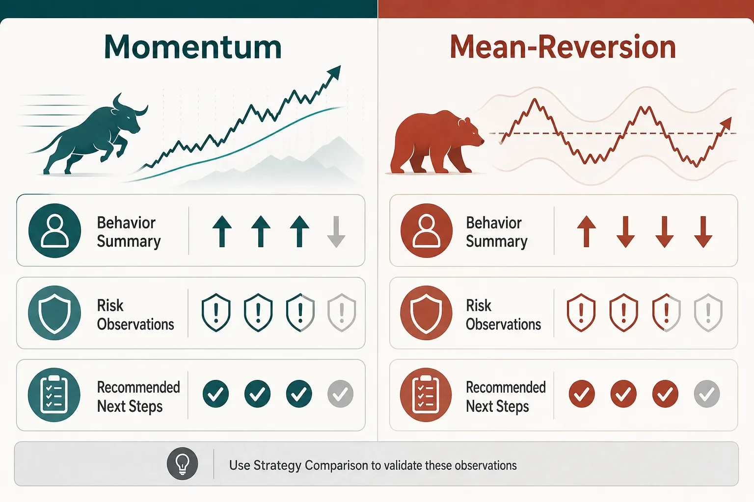
A step‑by‑step playbook for post‑event reviews: capture hypotheses, tag trades by catalyst, log outcomes, and use Strategy Comparison to see what held up during the Korea chip crash vs. Bitcoin rally.
 2026-08-11
How to Backtest Crypto Strategies Against Rising Rates and Oil Shocks — A Practical Template
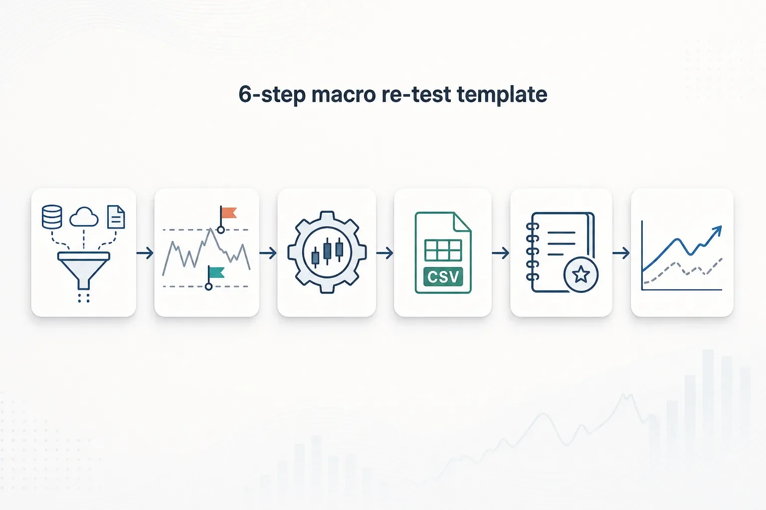
A hands-on template for re-testing crypto strategies when rates and oil spike: ingest macro time series, run variant backtests, record results in Trade Strategy, and compare outcomes to adapt sizing rules.
 2026-08-01
How Institutional Execution Tools Are Changing Prediction‑Market Trading — A Playbook for Quants
Talos’ institutional execution for Kalshi reduces friction for systematic prediction‑market strategies—but quants must add connectivity, execution simulation and monitoring. This playbook outlines practical steps and shows how Trade Strategy can document experiments today.